CAFOS in the Yucatán Peninsula

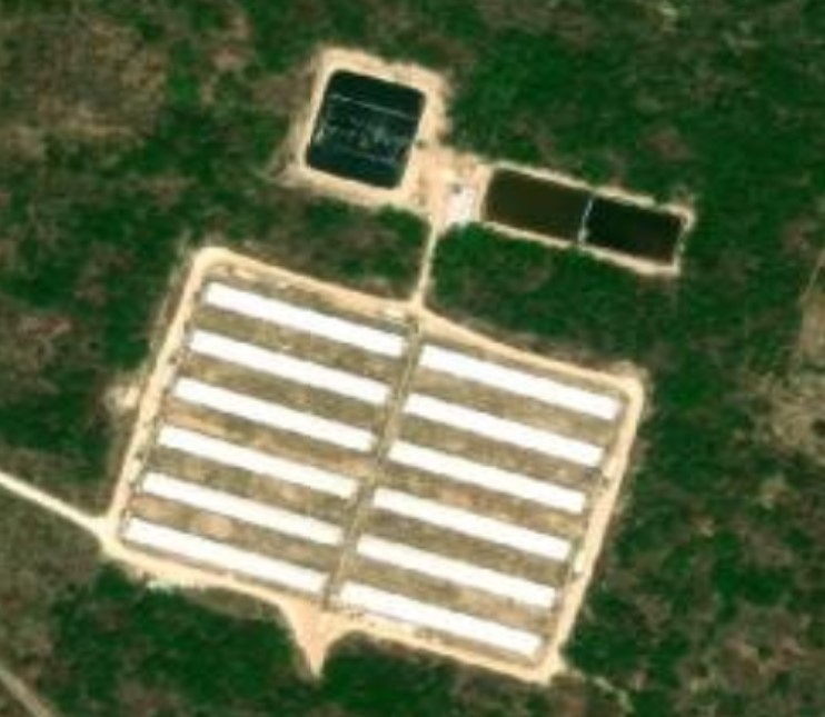
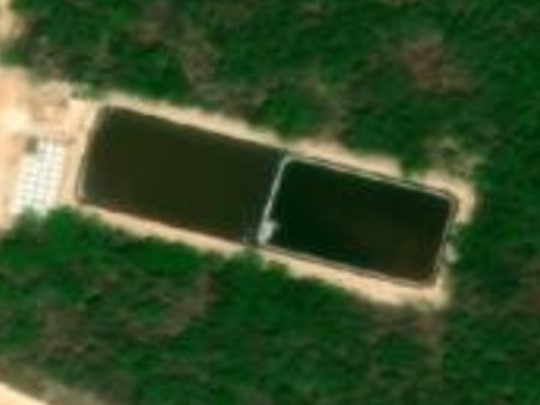
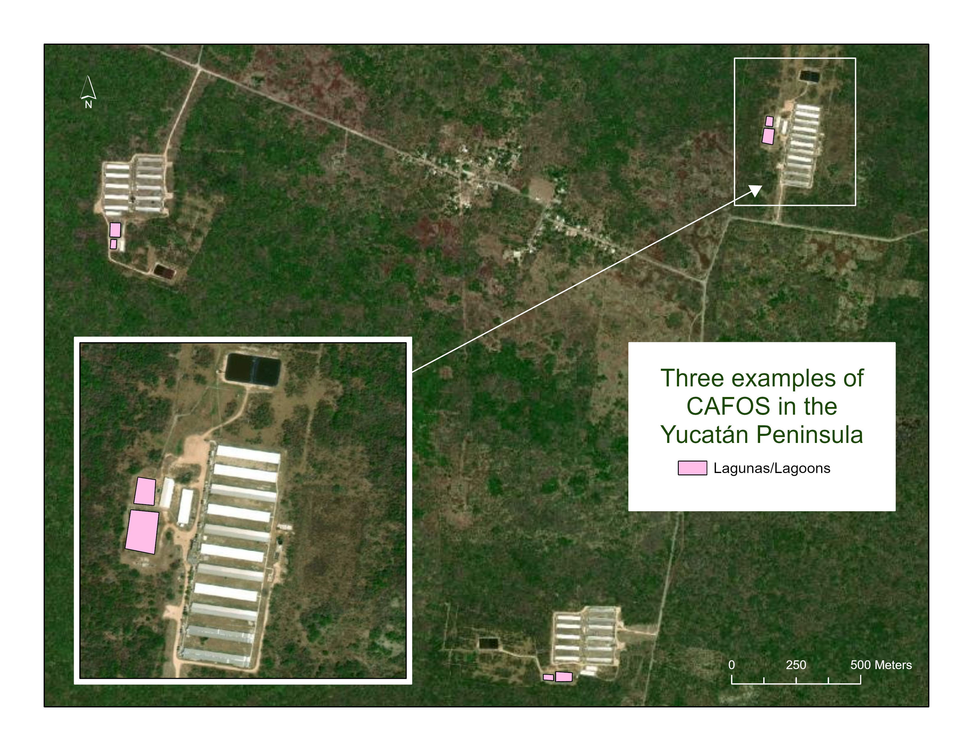
This project studied the growth of Concentrated Animal Feeding Operations (CAFOs) with André Luiz de Oliveira Domingues (Clark Universtiy, MSGIS) in Mexican’s Yucatán peninsula. CAFOS are intensive farming operations in which large numbers of pigs (in some cases up to 80,000 pigs) are held in indoor pens for meat production. Large amounts of fecal waste are generated from these animals and are disposed of in “lagunas,” or open pools of water and pig feces. These pens are breeding grounds for dangerous bacteria like Salmonella and E. coli and are not only unsanitary environments for the animals, but for communities living nearby.

Industrial pig farming has been growing in Mexico’s Yucatán Peninsula with adverse environmental and social impacts, including; the destruction of livelihoods (mainly due to environmental degradation), increased rates of asthma, cancer, premature births, low birth weights, deforestation, and overconsumption and contamination of water. In this project we built upon previous work by Karen Vazques Hudlet, Michael Cecil, and Manuel Llano and focused on studying the growth of CAFOs in the Yucatán peninsula using Rgee for RStudio and Landsat 8 and Sentinel 2 images from Google Earth Engine. We developed a method for identifying CAFO’s refuse lagoons from satellite imagery— as these lagoons have a unique spectral signature compared to other bodies of water— to identify when the lagoons first began to appear in the peninsula and at what scale and rate their number has grown over time. We used both Sentinels 2 and Landsat 8 satellite images in our analyses. We created an image collection for each year that included every image from the span of a few months (one image for each day) and used a cloud mask to remove cloud interference. We trained a Random Forest classifier for both Sentinel 2 images collections (2019-2022) and Landsat8(2014-2018) using spectral signatures from existing lagunas and sample polygons of “not lagunas” (polygons of mixed spectral signatures including, forest, urban, beach, etc.). We used our trained classifier to loop through each year to find and classify lagunas and represent the data in R with maps and graphs that show the distribution of CAFOS in the Yucatan Peninsula. We hope this information will aid in identifying and mapping CAFOS in Yucatan even if they are previously undocumented and will add to previous research on CAFOs in Yucatán and support community claims of increasing, illegal, industrial swine operations in their territories.

Software/Packages used: R Studio, GitHub, Random Forest, rgee (package API for GEE)

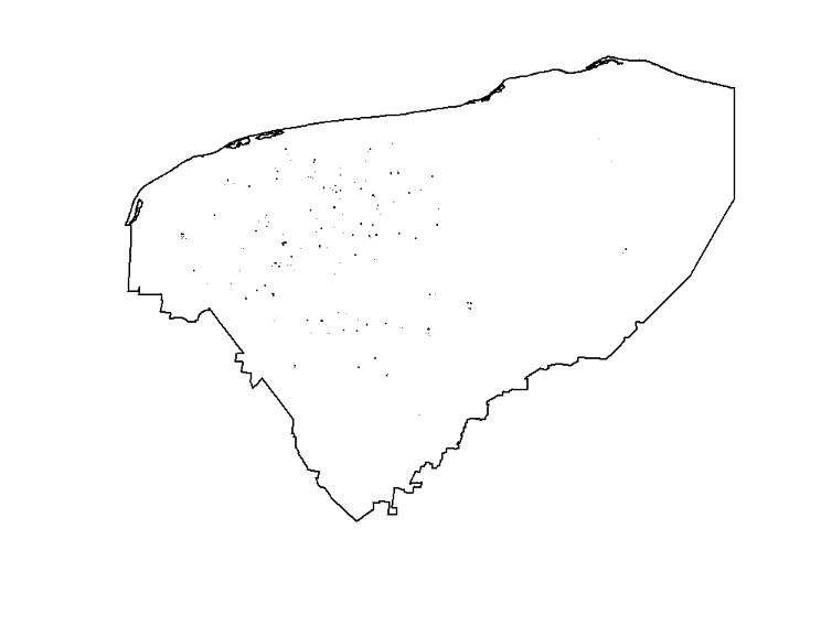
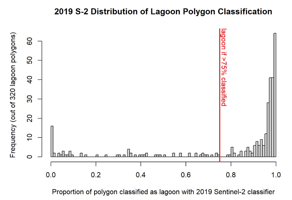
We tested various proportions to be used as the cut-off for which lagoon polygons should be classified as lagoon, before settling on 0.75 for Sentinel-2. We found that if we classified only known lagoon polygons that had at least 75% of their areas classified as lagoons, this maximized the number of known lagoons that we correctly classified and minimized how many we overclassified. The Landsat 8 classifier therefore misses a lot more lagoons than the Sentinel-2 classifier, which is why we went with a much more lenient cut-off proportion (5% vs 75%).

we created a function that extracts Landsat 8 composites of specified years and returns the number of classified CAFO lagoons for that year. Originally we tried to do it as a for loop to only have to run the code once, but R kept timing out.

# Function for counting Lagoons with L8
# parameters: 
#   year: year of landsat 8 image
#   proportion: proportion of lagoon area that needs to be classified as lagoon to be counted as lagoon.

# Define function name and parameters
L8_countLagoons <- function(year, proportion) {
  
  ## 1. Import Landsat 8 image for training classifier
  # Landsat 8 data: https://developers.google.com/earth-engine/datasets/catalog/LANDSAT_LC08_C02_T1_L2
  l8_image <- ee$ImageCollection('LANDSAT/LC08/C02/T1_L2')$
    filterBounds(yucatan_feature$geometry())$
    map(function(image){ image$clip(yucatan_feature) })$
    filterDate(paste0(year, '-01-01'), paste0(year, '-12-31'))$
    filter(ee$Filter$lt('CLOUD_COVER', 15))$
    map(maskL8sr)$
    median()$
    setDefaultProjection(crs = "EPSG:32616", scale = 30)
  
  ## 2. Add indexes & ratio to Landsat 8 compound image
  l8_image <- l8_addNWI(l8_image)
  l8_image <- l8_addNDWI(l8_image)
  l8_image <- l8_addEWI(l8_image)
  l8_image <- l8_5_4ratio(l8_image)
  
  ## 3. Classify Landsat 8 images using the trained RandomForest classifier:
  l8_classified <-l8_image$
    select(l8_bands)$                      # use the specified bands for classification
    classify(l8_trainedClassifier)         # use trained clasifier
  
  ## 4. Find average classification inside each lagunas_fc polygon:
  # Add reducer output to the Features in the collection.
  l8_proportionLagoon <- l8_classified$reduceRegions( # only band in the 2019 classified is the presence (0 or 1)
    collection = lagunas_fc,                  # original lagunas fc
    reducer = ee$Reducer$mean(),              # Average
    scale = 30
  )
  
  ## 5. Transfer fc to sf object to get a reliable count.
  l8_proportionLagoon_sf <- ee_as_sf(l8_proportionLagoon)
  
  ## 6. Select Lagoons that are less than 5% classified as lagoon.
  # Select rows with mean <= 0.05 and show only index and mean columns
  l8_lagClass_gte <- l8_proportionLagoon_sf %>%
    filter(mean >= proportion) %>%
    select(index, mean) %>%
    arrange(desc(mean))
  
  ## 7. Find number of lagoons in given year
  l8_num_lagoons <- nrow(l8_lagClass_gte)  # Number of lagoons classified more than 5% as lagoon.
  
  ## 8. Show distribution of % of classified lagoons
  # Create a histogram of the 'mean' column
  l8_lagoonClassDistro <- hist(l8_proportionLagoon_sf$mean, breaks = seq(0, 1, 0.01), 
  xlab = "Avg Classified", ylab = "Frequency", main = paste0("Count of Lagoons included in each classification tier for ", year))
  
  ## 9. Name variables with the year given in argument
  #rm(l8_avglagoon)
  assign(paste0("l8_", year), l8_image, envir = .GlobalEnv)
  assign(paste0("l8_classified_", year), l8_classified, envir = .GlobalEnv)
  assign(paste0("l8_proportionLagoon_sf", year), l8_proportionLagoon_sf, envir = .GlobalEnv)
  assign(paste0("l8_lagClass_gte", proportion, "_sf_", year), l8_lagClass_gte, envir = .GlobalEnv)
  assign(paste0("l8_num_lagoons_", year), l8_num_lagoons, envir = .GlobalEnv)
  assign(paste0("l8_lagoonClassDistro_", year), l8_lagoonClassDistro, envir = .GlobalEnv)
  
  ## 10.Print total lagoon count by year.
  paste0("In ", year, ", there were ", l8_num_lagoons, " CAFO lagoons in the state of Yucatán.")

  ### END
}